
Let’s take a look at how you can import star data into your projects using Python. This can be useful for creating your own star maps or decorative backgrounds. For this example, the positions will be plotted in a DXF file, as this is a common vector file format. Feel free to modify the code to export into your preferred format.
Star Position Data
This project demonstrates how to obtain the positions of stars visible from any location on Earth at any date and time between 1899-07-29 and 2053-10-09.
In order to limit the output, the stars are filtered by brightness (magnitude) to include only those visible to the naked eye.
Additionally, it shows how to filter stars by angle to exclude those obstructed by the horizon.
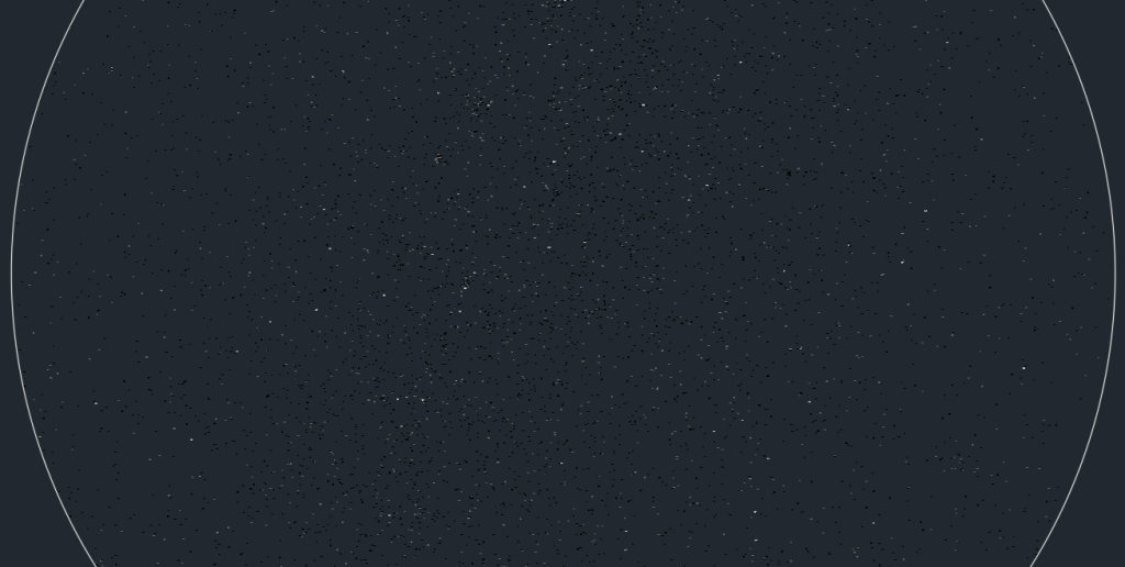
output
Using stereographic projection, the latitude and longitude of each star’s position are converted into X,Y coordinates for plotting on a 2D plane.
The stars are then plotted in DXF format, which is compatible with AutoCAD and many other vector graphic programs. However, any other format that uses X,Y positioning can be substituted.
The colour of the plotted points and labels varies with the brightness of the stars, making the brightest stars stand out more, similar to how they appear in the night sky.
Libraries and Initial Setup
First, let’s import the necessary libraries:
from skyfield.api import Topos, load
from skyfield.data import hipparcos
from skyfield.starlib import Star
import ezdxf
import math- Skyfield: A Python library for astronomy that allows you to compute positions for stars and planets.
- ezdxf: A library to create DXF files.
- math: Standard Python library for mathematical operations.
If any of the libraries are missing in your environment, you can install them using pip:
pip install skyfield ezdxfLoad Astronomical Data
We need to load the timescale and planetary data, which will be used to calculate the observer’s position and the star positions:
ts = load.timescale()
planets = load('de421.bsp')
earth = planets['earth']
Define Observer’s Location and Time
Specify the observer’s geographical location and the time of observation:
observer_lat = '51.503 N'
observer_lon = '-0.119 W'
observer = earth + Topos(observer_lat, observer_lon)
t = ts.now()
Latitude and longitude are set to the London Eye. Feel free to modify for your desired location. Time can be set to a fixed date and time by replacing it with this:
t = ts.utc(2024,1,2,3,4)This will set the time and date to January 2, 2024, at 03:04 UTC.
Load the Hipparcos Star Catalog
Load the Hipparcos star catalog, which contains data for over 100,000 stars:
with load.open(hipparcos.URL) as f:
  df = hipparcos.load_dataframe(f)
Filter Visible Stars
We filter the stars to only include those visible to the naked eye by setting a magnitude threshold. The lower the magnitude, the brighter the star:
magnitude = 7
visible_stars = df[df['magnitude'] < magnitude]

print(f"Number of stars: {len(visible_stars)}")
Create a DXF Document
We create a new DXF document where we’ll plot the stars:
doc = ezdxf.new('R2010')
msp = doc.modelspace()
Define the Stereographic Projection Function
We use a stereographic projection to map celestial coordinates to a 2D plane:
def stereographic_projection(lon, lat, lon_0=0, lat_0=90):
    lon = math.radians(lon)
    lat = math.radians(lat)
    lon_0 = math.radians(lon_0)
    lat_0 = math.radians(lat_0)

    sin_lat = math.sin(lat)
    cos_lat = math.cos(lat)
    sin_lat_0 = math.sin(lat_0)
    cos_lat_0 = math.cos(lat_0)
    cos_lon_diff = math.cos(lon - lon_0)

    k = 2 / (1 + sin_lat_0 * sin_lat + cos_lat_0 * cos_lat * cos_lon_diff)
    x = k * cos_lat * math.sin(lon - lon_0)
    y = k * (cos_lat_0 * sin_lat - sin_lat_0 * cos_lat * cos_lon_diff)

    return x, y
Define Colour Mapping Function
We map the star’s magnitude to a colour:
def get_dxf_color(value):
    if value <= (magnitude * 0.166):
        return 7
    elif value <= (magnitude * 0.333):
        return 254
    elif value <= (magnitude * 0.5):
        return 253
    elif value <= (magnitude * 0.666):
        return 252
    elif value <= (magnitude * 0.833):
        return 251
    else:
        return 250
Values from white to black are used to create a gradient that roughly represents the stars brightness.
Calculate and Plot Star Positions
We iterate through the filtered stars, calculate their positions using the stereographic projection, and plot them in the DXF document:
count = 0
for hip in visible_stars.itertuples():
    star = Star(ra_hours=hip.ra_hours, dec_degrees=hip.dec_degrees)
    astrometric = observer.at(t).observe(star)
    alt, az, distance = astrometric.apparent().altaz()

    if alt.degrees > 0:  # Check if the star is above the horizon
        count += 1
        x, y = stereographic_projection(az.degrees, alt.degrees)
        x_scaled = (x * 1000) + 2000
        y_scaled = (y * 1000) + 2000
        color_code = get_dxf_color(hip.magnitude)

        msp.add_point((x_scaled, y_scaled), dxfattribs={'color': color_code})

        text_height = (max(5, 10 - hip.magnitude)) / 10
        msp.add_text(f"HIP {hip.Index}", dxfattribs={'height': text_height, 'color': color_code}).set_placement((x_scaled, y_scaled))

msp.add_circle((2000, 2000), 2000)
With alt.degrees > 0, all stars above the horizon will be plotted. If you wish to account for obstacles such as houses and trees that block the full view of the horizon, simply increase the angle.
Add Metadata to the DXF File
We add additional information like the observation date, time, location, and number of stars as text in the DXF file:
texts = [
    f"Observation date: {t.utc_datetime().date()}",
    f"Observation time: {t.utc_datetime().time()}",
    f"Latitude: {observer_lat}",
    f"Longitude: {observer_lon}",
    f"Magnitude: < {magnitude}",
    f"Number of stars: {count}"
]

start_x, start_y = 50, 450
line_height = 25
for i, text in enumerate(texts):
    y_position = start_y - (i * line_height)
    msp.add_text(text, dxfattribs={'height': 20, 'layer': 'TEXT'}).set_placement((start_x, y_position))
Save the DXF File
Finally, we save the DXF file. Ensure you add the full export path to the file name:
doc.saveas(‘visible_stars.dxf')Conclusion
This script demonstrates how to import and visualize star data in a DXF format. By using the Skyfield library to handle astronomical data and ezdxf to generate the DXF file, you can automate the creation of intricate and accurate celestial designs. This approach can be tailored to specific needs, such as adjusting the magnitude threshold to control the number of visible stars, and can be executed efficiently in a matter of seconds.
This process can be particularly useful for custom applications like star sky roofs, decorative backgrounds, or any project that requires precise celestial mappings. Feel free to modify and extend this code to suit your specific requirements.
Complete code:
from skyfield.api import Topos, load
from skyfield.data import hipparcos
from skyfield.starlib import Star
import ezdxf
import math

# Load data
ts = load.timescale()
planets = load('de421.bsp')
earth = planets['earth']

# Observer's location
observer_lat = '51.503 N'
observer_lon = '-0.119 W'
observer = earth + Topos(observer_lat, observer_lon)

# Time of observation
t = ts.now()
#t = ts.utc(2024,1,2,3,4)

# Load the Hipparcos star catalog
with load.open(hipparcos.URL) as f:
    df = hipparcos.load_dataframe(f)

# Filter stars visible to the naked eye
#larger = more stars
magnitude = 7
visible_stars = df[df['magnitude'] < magnitude]


# Create a new DXF document
doc = ezdxf.new('R2010')  # Use the DXF R2010 format for compatibility
msp = doc.modelspace()

print(f"Number of stars: {len(visible_stars)}")

def stereographic_projection(lon, lat, lon_0=0, lat_0=90):
    # Convert degrees to radians for calculation
    lon = math.radians(lon)
    lat = math.radians(lat)
    lon_0 = math.radians(lon_0)
    lat_0 = math.radians(lat_0)

    # Compute the stereographic projection
    sin_lat = math.sin(lat)
    cos_lat = math.cos(lat)
    sin_lat_0 = math.sin(lat_0)
    cos_lat_0 = math.cos(lat_0)
    cos_lon_diff = math.cos(lon - lon_0)

    k = 2 / (1 + sin_lat_0 * sin_lat + cos_lat_0 * cos_lat * cos_lon_diff)
    x = k * cos_lat * math.sin(lon - lon_0)
    y = k * (cos_lat_0 * sin_lat - sin_lat_0 * cos_lat * cos_lon_diff)
    return x, y

def get_dxf_color(value):
    # Define a gradient of DXF colors from bright to dim stars
    if value <= (magnitude * 0.166):
        return 7
    elif value <= (magnitude * 0.333):
        return 254
    elif value <= (magnitude * 0.5):
        return 253
    elif value <= (magnitude * 0.666):
        return 252
    elif value <= (magnitude * 0.833):
        return 251
    else:
        return 250

count = 0
# Calculate positions for visible stars
for hip in visible_stars.itertuples():
    star = Star(ra_hours=hip.ra_hours, dec_degrees=hip.dec_degrees)
    astrometric = observer.at(t).observe(star)
    alt, az, distance = astrometric.apparent().altaz()

    if alt.degrees > 0:  # Check if the star is above the horizon
        count += 1
        # Using azimuth and altitude as longitude and latitude for the projection
        x, y = stereographic_projection(az.degrees, alt.degrees)

        # Scale coordinates for better visualization in DXF
        x_scaled = (x * 1000)+2000  # Scale factor for x
        y_scaled = (y * 1000)+2000  # Scale factor for y

        # Get color based on magnitude
        color_code = get_dxf_color(hip.magnitude)

        # Add point to DXF
        msp.add_point((x_scaled, y_scaled), dxfattribs={'color': color_code})

        # Calculate text height based on magnitude
        # Brighter stars (smaller magnitude) get larger text
        text_height = (max(5, 10 - hip.magnitude))/10  # Example scaling factor, adjust as needed

        # Add text label for the star name or HIP number
        msp.add_text(f"HIP {hip.Index}", dxfattribs={'height': text_height, 'color': color_code}).set_placement((x_scaled, y_scaled))

msp.add_circle((2000,2000),2000)
# Format a text string with the desired information
texts = [
    f"Observation date: {t.utc_datetime().date()}",
    f"Observation time: {t.utc_datetime().time()}",
    f"Latitude: {observer_lat}",
    f"Longitude: {observer_lon}",
    f"Magnitude: < {magnitude}",
    f"Number of stars: {count}"
]

# Define the initial position for the first line of text
start_x, start_y = 50, 450  # Top-left corner of the text block
line_height = 25  # Height of each line

# Add the information text to the DXF file
for i, text in enumerate(texts):
    y_position = start_y - (i * line_height)  # Move down for each new line
    msp.add_text(text, dxfattribs={'height': 20, 'layer': 'TEXT'}).set_placement((start_x, y_position))

# Save the DXF file
print(f"Number of plotted stars: {len(count)}")
doc.saveas('visible_stars.dxf')
Leave a Reply